Design Verification Challenge #1 - Maximize FIFO Queues on a 4-CPU Cache Controller Design

The Problem

The tremendous advances in Integrated Circuit (IC) Design has brought us great products over the last decade. These advances in IC's have also increased the complexity of Design Verification significantly. Design Verification (DV), the process of verifying that an IC functions as intended, takes up more than 50% of the time and cost of designing an IC (Reference: Research study by Siemens). Costs of DV are increasing, and, the time-to-market for new IC projects are slipping due to DV. To meet the growing demand for IC's we need to find innovative ways to speed up verification and reduce the associated costs. Additionally, as the research highlights, DV requires a significant amount of engineering talent and, the demand for DV Engineers grew at a 6.8% CAGR. There are not enough DV engineers being produced to meet this demand. Using innovative Machine Learning approaches presents significant opportunities to accelerate innovation in DV.

The Objective for the DV Challenge

The Objective of this DV Challenge is for participants to use innovative Machine Learning techniques to speed up verification and find bugs faster. The goal in this challenge is to maximize the average FIFO depths in a MESI Cache Controller Design. There are 4 FIFO Queues in this Cache Controller, one for each CPU. Each FIFO queue can hold up to 16 entries. The goal is to maximize the number of entries in each FIFO. Simply put, the higher average FIFO depth across all 4 queues the better are our chances of finding hard bugs. Participants can tune the Machine Learning Hyper-parameters and DV Knobs (settings) to increase the FIFO depths. VerifAI's Machine Learning Platform helps DV Engineers speed up verification. Finding bugs faster and Speeding up DV, reduces costs and improves time to market significantly.

What is a MESI Cache Controller

A Cache Controller makes sure that the data in the Cache and Main Memory are consistent (coherent). MESI (Modified Exclusive Shared Invalid) is a Cache Coherence Protocol widely used in Cache Controllers!

What is the FIFO (First In First Out) Queue

The job of a FIFO Queue is to store instructions or data in a queue, and service them later in the order they were entered into the queue.

Why fill up FIFO Queues

Filling up the FIFO queues activates parts of the design that are normally inactive. Bugs in deep states of the MESI Cache Controller design can only be found if the FIFO queues are filled. Therefore, maximizing FIFO depth , can find bugs that are normally hard to find.

How to fill up the FIFO Queues

It is hard to fill FIFO queues with random instructions and knob settings. A typical UVM DV Methodology generates random instructions, and may set random address ranges to try and fill the FIFO queues.
In this example, a DNN (Deep Neural Network) learns from an Initial Random (UVM) simulation and then generates the next set of instructions and addresses for the simulations. You can tune the hyper-parameters for the DNN so it learns to find the right knobs (features) that make the biggest difference in increasing the FIFO depth. After you tune the hyper-parameters, just click 'Optimize' and wait for the results. The higher your score the better.

Flow: What are we actually doing ?

In each iteration, input knobs are fed into the open-source Verilator simulator as stimulus, the simulator produces and output and we measure the associated FIFO depths reached for each CPU. These outputs and the inputs that were fed into the simulator are now fed into the VerifAI Optimizer, which is a Neural Network that predicts the next set of knobs for the simulator. In each iteration, the VerifAI Neural Network learns which input stimuli to the simulator produces the best output, highest FIFO depths in this particular case.

More about the MESI Cache Controller

The design is an open-source MESI Cache Controller, that has 4 CPU's.The Cache Controller design is an opensource design from opencores.org and its licensed under LGPL. The Cache Controller design is shown in Figure 1.The controller supports up to four CPUs. Each CPU has its own FIFO of depth 16. FIFO's are used to resolve load-store conflicts. For example, if multiple CPUs try to access the same address at the same time, the CPU with higher priority gets the access and the CPU with lower priority will insert the access request into its FIFO queue. These requests are serviced at a later time. It is hard to fill FIFO queues with random traffic, since only address conflicts cause entries to be inserted into the queues.
       In this experiment, we use the open source simulator Verilator that drives the VerifAI Machine Learning based Optimizer. The Optimizer produces the next set of knobs for the simulator to improve the FIFO depth.

DV Knobs to Tune

The DV Knobs exposed in this design are shown below. You can set these percentages to generate the initial random knob settings for the simulations. The knob settings are to create the initial randomized settings that are used as the inputs to the simulator.

• No. of Simulations -- Specify the number of simulations that should be run per iteration of the optimizer, each simulation represents one row in a CSV file, with settings for each of the knobs shown below. The default is 100 simulations.
• Knobs to control the Instructions:
• % Read (recommend the relative distribution for Read Instructions)
• % Write (recommend the relative distribution for Write Instructions)
• % RdBroadcast (recommended weights for ReadBroadcast Instructions)
• % WrBroadcast (recommended weights for WriteBroadcast Instructions)
• Knobs to control Memory Address - Tag, Index and Offset ranges for each CPUs
• The Tag portion of the address (address bits 31:16) is forced to a maximum range specified by:  { 0 : 0x0001, 1 : 0x0002, 2 : 0x0004, 3 : 0x0008, 4 : 0x000F, 5 : 0x00FF, 6 : 0x0FFF, 7 : 0xFFFF}
• The Index portion of the address (address bits 15:4) is forced to a maximum range specified by: { 0 : 0x000, 1 : 0x001, 2 : 0x002, 3 : 0x004, 4 : 0x008, 5 : 0x000F, 6 : 0x0FF, 7 : 0xFFF}
• The Offset portion of the address (address bits 3:0) is forced to a maximum range specified by:  { 0 : 0x1, 1 : 0x2, 2 : 0x4, 3 : 0x8, 4 : 0xA, 5: 0xB, 6 : 0xC, 7 : 0xF}

Hyperparameters to Tune

• Optimizer (Choose the optimizer type from the list to use on the Deep Neural Network). Each optimizer uses a slightly different algorithm to converge, i.e. minimize the given loss function and try to find a local minima. The most common optimization algorithm is know as Gradient Decent. The algorithms specified here are some variant of a Gradient Descent algorithm. A list and description of all the optimizers is given here in the Keras documentation.
• Loss Function (Choose the loss function you want to use for the optimizer). A list of loss functions is given here in the Keras documentation. The purpose of the loss function is to compute a quantity, that will be minimized by the optimization algorithm during training of the Neural Network
• Hidden Units (Specify the architecture of the hidden layers of the DNN). The hidden layers are the intermediate layers between the input and the output layers of a DNN. The hidden layers are typically determine how quickly and accurately the Neural Network will learn function that predicts the outputs from the inputs. The 'Deep' in Deep Learning refers to the depth of the hidden layers in a Neural Network. The depth of the Neural network is the number of hidden layers plus 1.
• Training Epochs (Specify the number of training epochs). One epoch consists of one training iteration on the training data. When all samples in the training data is processed, the second epoch of the training begins, and so on. The number of epochs plays a role in the DNN converging and reducing losses.
• Batch Size (Specify the batch-size for the dataset). The dataset is broken up into mini-batches and passed into the Neural Network to be trained. The batch size determines how many rows of data are processed at one time thru the Neural Network. For instance, if you have 1000 training samples and you use a batch size of 100, the training algorithm will take in the first 100 samples , next it will take samples from 101 to 200 and train the network again, till all the data samples are trained through the Neural Network.
• Iterations (Specify the number of times to iterate between the simulations and the optimizer). This parameter specifies the number of iterations that the simulator output should be fed into the DNN to be trained. Each time the output of the simulator is fed into the DNN, the DNN returns back a set of predicted knobs for the next iteration of the simulations, that will maximize the FIFO depths (in this case). The DNN learns to fit a function that mimics the effect of the simulator. Typically the higher the number the iterations, the better the predictions. But after a certain number of iterations, the DNN saturates, and does not get any more accurate.
• Ensemble Size (Specify the number of DNN's to create as an Ensemble Network). Ensemble learning is a method that uses multiple DNN's to improve prediction of individual networks. Using ensemble networks produces more accurate learning networks, but this comes at the cost of runtime.

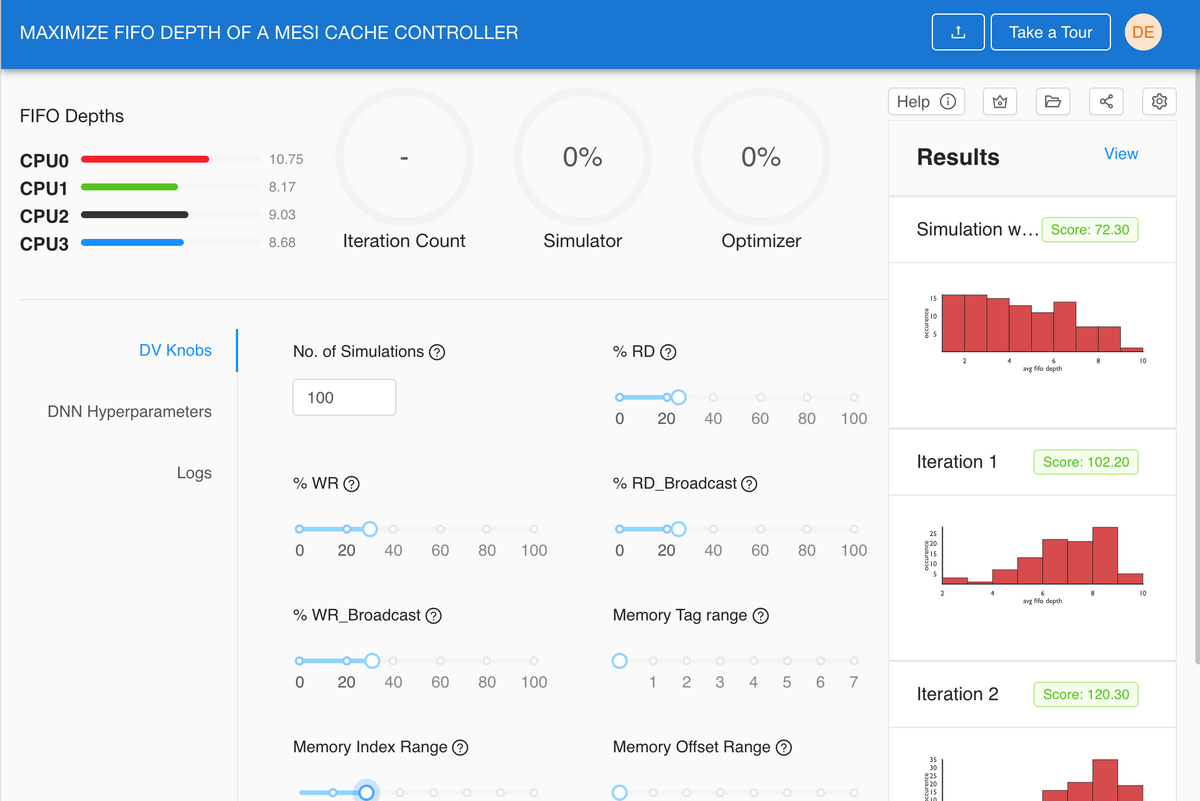
Results: What to expect

As mentioned above the goal of this experiment is to tune the initial knobs to generate a weighted random distribution of stimulus for the simulator. The Hyper-parameters are used to tune the DNN (Deep Neural Network) to produce the highest average FIFO depths. Each iteration should move the histograms distributions to the right, such that there are higher number of occurrences for higher FIFO depths.

The final score of your results is calculated as a weighted sum of the histogram distribution. This histogram has 16 bins: An example calculation:

• Weights = [0.1, 0.2, 0.3, 0.4, 0.5, 0.6, 0.7, 0.8 , 0.9 , 1.0, 1.1, 1.2, 1.3, 1.4, 1.5, 1.6]
  
• Example: histogram = [16, 29, 24, 13, 8, 1, 1, 0, 0, 1, 0, 1, 2, 2, 0, 1]
  
• Score = (histogram * Weights).sum() : The score is computed by the sum of dot product of the weights and the histogram values
                     The higher the score the better. The leaderboard shows the top scores of other users who have run the FIFO optimizer.
  

The Histogram below shows the distribution of the average FIFO depths. The goal is to shift the distribution to the right, to get higher occurrence of larger FIFO depths.

FIFO Challenge WebPage